Office 2016 For Mac Add Secondary Axis

How to create combination charts and add secondary axis for it in Excel?

Add or remove a secondary axis in a chart in Office 2010. When the values in a 2-D chart vary widely from data series to data series, or when you have mixed types of data (for example, price and volume), you can plot one or more data series on a secondary vertical (value) axis.

In Excel, we always need to create charts comparing different types of data. There are several chart types we can use, such as column, bar, line, pie, scatter chart and so on. Sometimes it's necessary to plot two or more sets of values to show multiple types of data, such as a column chart and a line graph. In this case, you can create a combination chart which is to combine two different charts to make one (see following screenshots). Today, I will talk about how to create combination charts and add a secondary axis as well in Excel.

• Reuse Anything: Add the most used or complex formulas, charts and anything else to your favorites, and quickly reuse them in the future.
• More than 20 text features: Extract Number from Text String; Extract or Remove Part of Texts; Convert Numbers and Currencies to English Words.
• Merge Tools: Multiple Workbooks and Sheets into One; Merge Multiple Cells/Rows/Columns Without Losing Data; Merge Duplicate Rows and Sum.
• Split Tools: Split Data into Multiple Sheets Based on Value; One Workbook to Multiple Excel, PDF or CSV Files; One Column to Multiple Columns.
• Paste Skipping Hidden/Filtered Rows; Count And Sum by Background Color; Send Personalized Emails to Multiple Recipients in Bulk.
• Super Filter: Create advanced filter schemes and apply to any sheets; Sort by week, day, frequency and more; Filter by bold, formulas, comment..
• More than 300 powerful features; Works with Office 2007-2019 and 365; Supports all languages; Easy deploying in your enterprise or organization.

Create combination charts in Excel

Supposing you have the following two data sources, you can create combination charts based on the data source with these steps:

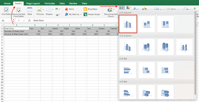
1. First, we can create a column chart for the first Area data source, please select the data range and then specify a column type chart under Insert tab, and then a column chart will be created as following screenshots shown:

2. Then select the Total Price data range, press Ctrl + C to copy it and then click any column in the above column chart, press Ctrl + V to paste the data into the chart. Now we have a column chart with two data sets (Area and Total Price), both charted using the same chart type. See screenshot:

3. In this step, we need to change one of the data sets to a line chart. Please click red bar Total Price data column in the chart, and right click, then choose Change Series Chart Type from the context menu, see screenshot:

4. In the Change Chart Type dialog, select one line chart type as you need, see screenshot:

5. Then click OK button, and now you have a chart with two chart types as following screenshot shows:

Note: With repeating above steps, you can combine more than two chat types, you just need to select the additional data sets and choose a different chart for each data series.

Add a secondary axis for the combination charts

Sometimes, in a combination chart, the values of one data set vary widely from another, so it is difficult for us to compare the data from the chart. To make the chart easier to read, Excel allows us to add a secondary axis for the chart, here’s how you add a secondary axis for the combination chart in Excel.

1. In the combination chart, click the line chart, and right click or double click, then choose Format Data Series from the text menu, see screenshot:

2. In the Format Data Series dialog, click Series Options option, and check Secondary Axis, see screenshot:

3. Then click Close button, and you have successfully added a secondary axis to your chart as following screenshot:

Related articles:

• Reuse: Quickly insert complex formulas, charts and anything that you have used before; Encrypt Cells with password; Create Mailing List and send emails..
• Super Formula Bar (easily edit multiple lines of text and formula); Reading Layout (easily read and edit large numbers of cells); Paste to Filtered Range..
• Merge Cells/Rows/Columns without losing Data; Split Cells Content; Combine Duplicate Rows/Columns.. Prevent Duplicate Cells; Compare Ranges..
• Select Duplicate or Unique Rows; Select Blank Rows (all cells are empty); Super Find and Fuzzy Find in Many Workbooks; Random Select..
• Exact Copy Multiple Cells without changing formula reference; Auto Create References to Multiple Sheets; Insert Bullets, Check Boxes and more..
• Extract Text, Add Text, Remove by Position, Remove Space; Create and Print Paging Subtotals; Convert Between Cells Content and Comments..
• Super Filter (save and apply filter schemes to other sheets); Advanced Sort by month/week/day, frequency and more; Special Filter by bold, italic..
• Combine Workbooks and WorkSheets; Merge Tables based on key columns; Split Data into Multiple Sheets; Batch Convert xls, xlsx and PDF..
• More than 300 powerful features. Supports Office/Excel 2007-2019 and 365. Supports all languages. Easy deploying in your enterprise or organization. Full features 30-day free trial. 60-day money back guarantee.

• Enable tabbed editing and reading in Word, Excel, PowerPoint, Publisher, Access, Visio and Project.
• Open and create multiple documents in new tabs of the same window, rather than in new windows.
• Increases your productivity by 50%, and reduces hundreds of mouse clicks for you every day!

• To post as a guest, your comment is unpublished.
  Is there any way to put a real scale in horizontal axis?
  Here, datas are equally distanced from each other, I would like to put a horizontal numerical axis and actually have the real distance between datas.
  Do you know a way to do it in Excel?
  I hope I was clear enough.. Thank you!
• To post as a guest, your comment is unpublished.
  Good job.really helped
• To post as a guest, your comment is unpublished.
  You can actually create a dual axis chart in DataHero automatically by dragging two numeric attributes onto the chart. It saves you a lot of steps in Excel.
• To post as a guest, your comment is unpublished.
  creating a pareto chart

When using Excel and working with two data sets that differ greatly in range it can be difficult to chart those values due to the larger range of one of your data sets. A classic example of this would be your monthly data and your YTD values for each month. When you put these together in a chart the monthly data is diminished by the much larger YTD values. In order to overcome this you can assign each data set an axis.

The default for all your data sets is the Primary axis, you have the option of assigning your second data set to the second axis which makes your chart readable. Below you will find the instructions on how to add a second axis to an Excel graph.

If you have any comments or questions, please post them below.

Note: I used Excel 2003 for this demonstration, but it should hold true for 97-2007.

Graph without Second Axis

The following steps were written assuming you have a chart in excel with more than one data set.

If you wish to view the step-by-step, click the pic tutorial icon -> or you can follow the steps below.

1. Select a point on the graph for the data set you want to put on the secondary axis.

Amplitude Crack is an extremely valuable and flexible tool and can be used as a sophisticated multi-effects processor in its stand able version.

2. Right-click and select Format Data Series…

3. Click on the Axis tab and select the Secondary axis radio button

4. Click OK

5. Your selected data set should now reside on the second axis of your chart.

Graph with Second Axis Enabled